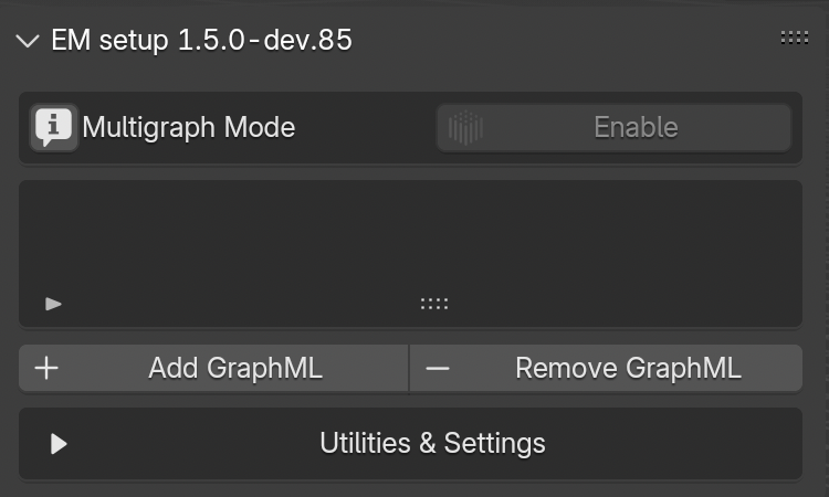
This panel (Fig. 44) allows to create the first connection between Blender and the Extended Matrix (.graphml file).
Press the AddGraphML and locate the .graphml file wiin the Path section (NB: before closing the path window remember to uncheck relativepath within the settings.
Alternatively, it is possible to paste the entire path within the empty line).
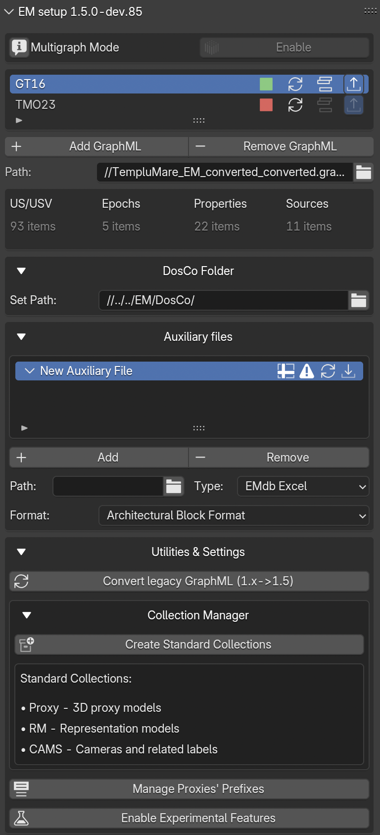
When a GraphML is loaded (Fig. 45), on the left side of the EM Data Tree window the GraphML ID will appear (for example, the ID: GT16).
On the same line, on the right side, a green square will show up.
The green color cofirms that a connection between the GraphML and EMtools has been established.
Note
To correctly link the .graphml file with the EMDataTree panel it is mandaotry to insert, at least, the GraphML ID on the title of the Swimlanenode (1.5 dev4 palette); the first node that needs to be imported in the yEd space to start the creation of an Extended Matrix (Fig. 46).
Next to the green (or red) square, three buttons complete the right side of the line (Fig. 45): the Update button allows to refresh the .graphml file, if changes have been applied on the EM graph during the modelling session; the ActivateEM button consent to explore only the selected GraphML; and the pubblish button appears when the multigraph mode is enabled.
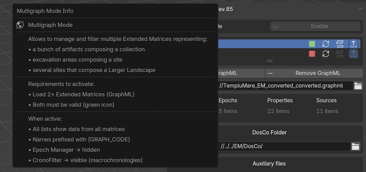
This version of EMtools allows to activate the MultigraphMode, this option consent to upload and visualize multiple graphs.
To upload a new graph and explore its information user can follow all the steps already explained.
Note
This version of EMtools include info boxes.
When the info button is selected an info box will appears with more information related to that specific part of the tool.
Once the connection has been established, EMTools will summarize the most important information (US/USV; Epochs; Properties; Sources) within a simple table under the Path section (Fig. 45).
The RemoveGraphML button allows to remove one or more EMs from the EM Data Tree list.
Note
Loading DosCo documents into the graph
The panel commands described below load documents from your DosCo
folder into the EM graph as nodes. The link between the file on
disk and the graph node is preserved; if you re-iterate your
DosCo (add new entries, update existing ones), reload from this
panel to surface the changes. For the DosCo concept, folder layout
and iteration pattern, see Iterating the DosCo in the Extended Matrix language manual.
In this panel (Fig. 45) users can also link the path to the DosCo folder, where sources are stored.
To locate sources, users must follow the same guidelines previously outlined for the localization of the EM file.
If the EM graph presents a connection with and external database, EMTools allows to import databases to maintain data connection also within Blender.
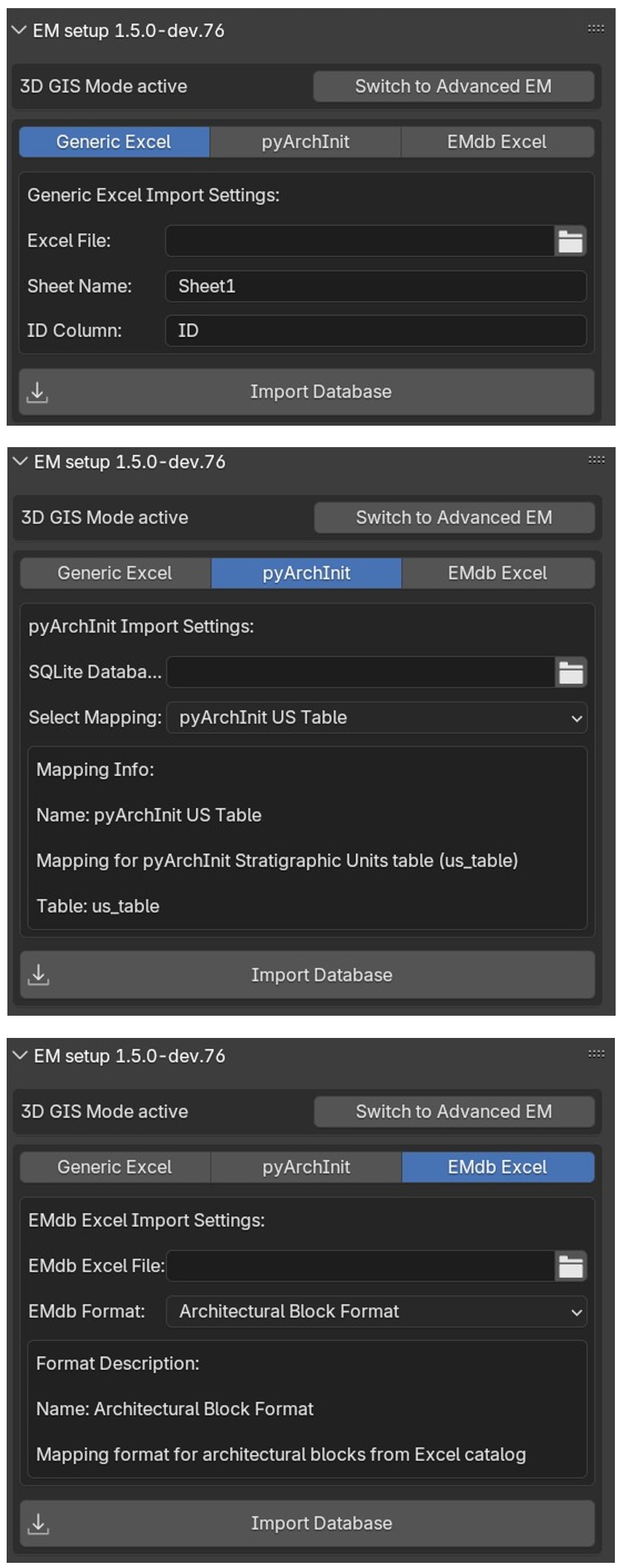
To establish the connection with EMtools:
expand the Auxiliaryfiles section and press Add;
select the type (Generic Excel, PyArchInit, EMdb Excel);
indicate the exact location of the Auxiliary file and click on the Accept button.
Note
When EMdb Excel type is selected a Format menu appears, select the correct format from the list.
Auxiliary files are not part of the EM graph’s core structure.
The graph (.graphml) defines stratigraphy, proxies, sources and
their logical relations; auxiliary files provide additional,
tabular information that EMtools attaches to existing graph nodes
at import time. They live outside the graph and can be re-imported,
re-mapped or detached without altering the topology of the
reconstruction.
The three currently supported auxiliary types behave the same way
conceptually but differ in their source format:
Generic Excel — any .xlsx with a header row; mapping is
defined by the user.
EMdb Excel — a tabular database structured according to the
EMdb conventions; mapping is driven by a JSON mapping file
(see JSON mapping template below).
Important
Auxiliary files in this sense (tabular data attached at import
time via a mapping) must not be confused with auxiliary
stratigraphic nodes in the EM language — Continuity and
related node types that belong to the formal notation. The
former is a data plumbing feature of EMtools; the latter is a
modelling primitive of the language. See the EM language
manual for the latter.
Typical use cases:
enrich existing US/USV nodes with material qualia, dating
ranges, excavator notes that live in a separate spreadsheet;
link photo paths and metadata to stratigraphic units without
redrawing the graph in yEd
(see Linking Photos as Auxiliary Files for the step-by-step procedure);
merge field-database records (pyArchInit) into an already
authored graph.
For the EMdb Excel (and Generic Excel) auxiliary types,
EMtools consumes a JSON mapping file that declares how each column
of the spreadsheet should be projected onto graph properties.
A minimal mapping has the following shape:
Each row of the spreadsheet (from start_row onward) is matched
against an existing graph node via id_column. For each entry
in mappings, EMtools writes the value of the indicated column
onto the target property of the matched node (or creates the
property if absent). Supported type values mirror the kinds of
data the EM language recognises (identifier, node_type,
epoch, qualia, document_link, …); the exact list
depends on the importer in use and is documented alongside the
operator in API Reference.
Todo
Ship a canonical emdb_mapping.template.json next to the
addon and reference it here once finalised. Until then the
shape above is the reference; live working examples can be
inspected in the Basilica Iulia dataset used by
Bulk Import via the Excel Mapping Tool.
Starting from version 1.5, EMtools allows to link external resource folders containing photos, 3D scans, documents and other media files to your Extended Matrix project.
This feature is particularly useful when working with large image collections that need to be referenced and previewed directly from within Blender.
Once a resource folder is configured, EMtools can automatically generate thumbnail previews of all images in that folder.
The thumbnail system creates a local cache that speeds up image browsing and reduces memory usage.
How it works:
Thumbnails are stored in a folder named EM_thumbs/ next to your .blend file
Each resource folder gets its own subfolder (e.g., Resources_abc12345)
The system remembers which images have been processed to avoid duplicates
If you sync your project via cloud storage, thumbnails are automatically shared across computers
In the Auxiliary Files panel, locate the text Thumbnailsfortheresourcefolder?Clickbelow.
Click the (Re)generatethumbnails button
EMtools will scan all images in the resource folder (including subfolders) and create previews
Progress information is displayed in the Blender console
The line Thumbs:Resources_xxxxxxxx shows the name of the cache folder that was created
Note
Supported image formats: JPG, PNG, BMP, TIFF, PDF (first page)
The generation process only creates thumbnails for new or modified images.
If you click (Re)generate again, existing thumbnails are skipped automatically.
A third section, the Utils sub-panel (labelled Utilities & Settings
in older builds), is included within the EM Data Tree panel.
Here, users can: convert an EM made with an old version of the formalism,
create the default collections, rename Proxies and enable Experimental
Features.
In the first case (Convert1.x->1.5 button) EMtools will normalise
older GraphML files authored with the 1.x palette to the 1.5 visual
conventions — see Convert 1.x->1.5 below for details.
Within this section, EMtools includes also a button, CreateStandardCollections, that allows to automatically create the set of default Blender collections used by a reconstruction workflow with Extended Matrix. The collections are:
Proxy — holds proxy meshes (volumetric placeholders for each US / USV / SF in the graph).
RM — holds Representation Models (the 3D reconstructions that visualise each US / USV).
RB — sub-collection under RM for reality-based RMs: photogrammetry, laser scan, drone-imagery and other reconstructions derived from a captured surface.
SB — sub-collection under RM for source-based RMs: hand-modelled reconstructions built from textual, iconographic or archaeological sources.
New in EM Tools 1.6.0-dev.8. The two sub-collections are created empty; the user moves meshes into the appropriate one by drag-and-drop in the outliner. A future patch may auto-route on promote_to_rm.
Layouts — holds camera + label setups for authoring 2D plates and publication figures. Renamed from ``CAMS`` in EM Tools 1.6.0-dev.8. The previous name was a Blender-ism (cameras for renders) that obscured what the collection actually holds; “Layouts” reflects the workflow purpose. Lookups across the addon prefer the new name and fall back to CAMS so projects authored against earlier builds keep working without a manual migration step.
By pressing ManageProxies'Prefixes button, EMtools will automatically rename Proxies according to the GraphML ID (NB: this step is mandatory to mutually connect GraphML and Proxies. User must select geometries before applying the tool).
By pressing the EnableExperimentalFeatures button, a set of Experimental Features will be activated within the sections of the EM Data Tree panel (Fig. 48).
The Convert1.x->1.5 button in the EM Data Tree → Utils
sub-panel migrates older Extended Matrix GraphML files (authored
with the 1.x generation of the yEd palette) to the 1.5 visual
conventions used by the current importer and tooling.
The button drives the graphml.convert_borders operator, which
reads a .graphml file and rewrites its node visual attributes
in-place on a new file:
Sets the border width to 4.0 for the EM target shapes
(rectangle, hexagon, ellipse, octagon, parallelogram).
Applies the 1.5 canonical border colours based on shape type
and background:
rectangle → #9B3333 (US / negative units)
hexagon → #31792D (USV)
ellipse → #31792D (USV variants)
parallelogram → #248FE7 (documents / extractors)
octagon → #D8BD30 (Special Find) when on a light background,
#B19F61 (Virtual Special Find) when on a black background.
The result is written next to the original file with a
_converted.graphml suffix; the source file is left untouched.
Select the legacy .graphml file and confirm. EMtools
produces <name>_converted.graphml in the same folder and
reports the output path in the Blender status bar.
Load the converted file with AddGraphML as you would any
other graph (see the Loading DosCo documents into the graph
note above for the load workflow).
The operator is a visual / palette normaliser, not a full
datamodel migration. In particular:
It does not invent or upgrade paradata. If the older graph lacked
family / is_series attributes on extractors and combiners,
the converted file reflects the same absence.
It does not rename relation edges whose semantics changed between
releases (e.g. is_after direction canonicalisation introduced
in v1.5.3). Such edges are preserved as-is and may surface as
importer warnings.
It does not re-link external documents. DosCo references in the
original are preserved as identifiers; ensure the corresponding
files are reachable in your DosCo folder.
For projects authored before EM 1.0 (pre-formalisation,
free-form yEd), conversion is not reliable: the original is best
used as a visual reference for manually rebuilding the graph in
the current palette.
For the missing pieces above, the importer side picks up some of
the slack: s3dgraphy.importer.import_graphml is forgiving on
older label conventions and re-maps known legacy types on the fly
during import, and the post-import passes in s3dgraphy.transforms
(hoist_propagative_metadata, prune_redundant_propagative_edges,
compact_propagative_metadata) can be used to normalise paradata
attribution programmatically.
A single, end-to-end s3dgraphy.utils.convert_legacy_em_graph
wrapper that combines the palette-normalisation step performed by
this button with the in-memory cleanup transforms is on the
s3dgraphy roadmap. Until it lands, the procedure above (button →
load → optional transforms → re-export) is the recommended path.
The anchor for this section (convert-legacy-em-graph) is
stable and will continue to point here when the wrapper is
published.
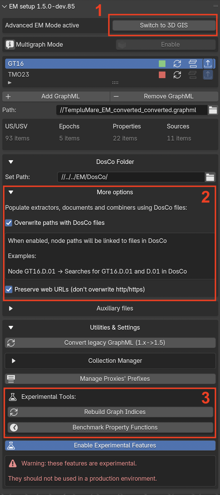
Fig. 48 Experimental Features enabled (red rectangles with numbers 1-3)
Note
As highlighted in the red warning, this set of features is experimental and it should not be used within the regular documentation process of the EM (Fig. 48).
Here a brief presentation of the Experimental Features, the numebers on the list refer to the numbers specified in Fig. 49:
On the upper part of the panel the Switchto3DGIS button allows to instantly switch from the EMmode to a 3DGISmode where users can link an external database to EMtools (Fig. 49). The activation of the 3DGISmode consents to connect an External database to the 3D environment of Blender via EMtools. User have three different type of external databases (Generic Excel, PyArchInit, EMdb Excel) to choose from. By pressing the corresponding button a diverse set of options will appear. After setting all the required information the external db will be import within EMtools.
Within the DosCoFolder section (Fig. 48) the Moreoption menu appears, this new part of the add-on permits to populate Extractors, documents and Combiners using DosCo files.
In the Utilities&Settings (Fig. 48) the activation of the EnableExperimentalFeatures button activates the ExperimentalTools section with RebuildGraphIndices, BenchmarkPropertyFunctions, and the collapsible Create a GraphML wizard.
Create a GraphML: A 3-step panel-based wizard for generating Extended Matrix GraphML files from Excel data — either filled manually using downloadable templates or produced by AI-assisted extraction from archaeological reports. The wizard works entirely in memory until export:
Step 1 — Convert Stratigraphy: Loads stratigraphy.xlsx (24-column template) and creates an s3dgraphy graph in memory.
Step 2 — Enrich with Paradata (optional): Loads em_paradata.xlsx and adds per-property provenance chains (PropertyNode → ExtractorNode → DocumentNode) to matching nodes.
Step 3 — Export GraphML: Saves the graph to a .graphml file. Import this file via File > Import EM file to populate the Blender scene.
The panel also provides template download buttons and an AI Extraction Prompt section with a language selector and a one-click Copy AI Prompt to Clipboard button.
Warning: This feature is experimental. Always verify the generated GraphML before using it in production.
When importing data from a PyArchInit SQLite database (and other
mapped tabular sources) through the 3D GIS mode, EMtools can filter
rows on the fly so you import only the subset you care about —
for example, one archaeological site at a time instead of every
site recorded in the database.
This works by reading the is_filter flags in the mapping JSON
file you select. For each column the mapping marks as filterable,
EMtools queries the database for the distinct values present and
populates a dropdown in the 3D GIS panel.
A database file in the DB field (the
pyarchinit_db_path property), and
A mapping (for example pyarchinit_us_mapping),
EMtools reads the mapping, finds columns marked is_filter:true,
and renders a box titled “Filter rows by:” with one dropdown
per filterable column. If the mapping has no filter columns the box
does not appear and the panel behaves exactly as in 1.5.
Up to 5 filter columns per mapping are supported. Beyond that
limit the extra columns are silently ignored.
A dropdown whose label ends with an asterisk (for example
Site*) is required: you must pick a specific value before
importing. The (Allvalues) placeholder is absent for these.
A dropdown without an asterisk is optional: choose
(Allvalues) to skip it (no filter applied on that column), or
pick a specific value to constrain the import.
Multiple filters combine with logical AND. For example, picking
Site=Pompei and Area=A imports only rows where both
conditions match.
Values are matched exactly — case-sensitive string equality.
There are no wildcards, ranges or multi-select.
Click Import. EMtools collects your dropdown choices into a
filters dictionary and passes it to the importer:
If a required filter was left at (Allvalues), the import is
aborted with an error message — pick a concrete value and retry.
If all required filters are set, the importer issues a SQL query
with a WHERE clause built from your selections
(parameterised, so the values are safely escaped).
Only rows matching the filters become nodes in the resulting
graph; everything else stays in the database, untouched.
Distinct values for a filter column are queried lazily, the first
time the dropdown is opened, and cached keyed on
(filepath,filemtime,columnname). Re-opening the dropdown
is therefore instant; changing the file on disk invalidates the
cache on the next read.
If you change the database path or the mapping in the
panel, EMtools resets all 5 filter slots and re-discovers the
filterable columns from scratch.
Filtering applies to the 3D GIS import path (the main
pyarchinit_db_path field shown in the 3D GIS panel). The
auxiliary-files import path described in
Auxiliary files — concept does not show filter dropdowns in
1.6 — it still imports the whole table.
If the mapping declares a filter column but the database table
is missing that column, the dropdown shows an error message
and the import is aborted. Fix the mapping (or the database
schema) and retry.
Filtering does not affect relations resolution: if you filter
out US #42 but US #38 has a relation pointing to #42, the
relation is dropped because the target sits outside the imported
subset. Workarounds: include both ends of the relation in your
filter, or re-import with a broader filter and prune the result
externally.
Starting with EM Tools 1.6, the pyArchInit 3D GIS import path
can read directly from a live PostgreSQL / PostGIS database in
addition to the historical SQLite file mode. This is the backend
real archaeological projects use in the field — multi-user editing,
QGIS-friendly geometry storage, server-side backups — so connecting
to it without exporting a SQLite snapshot first removes a whole step
from the daily authoring loop.
Scope — 3D GIS mode only (for now)
Everything described in this section applies specifically to the
3D GIS mode of the EM Setup panel (the Switchto3DGIS
workflow described above). In pure EM mode the data
ingestion goes through a different code path that does not yet
use the PostgreSQL/PostGIS backend introduced here — pure-EM
projects still consume their source data through the existing EM
importers. Bringing the same backend into pure EM mode is on the
roadmap but is not part of this release. Until then, the
one-click “live database” experience is a 3D GIS feature.
Contributed by Enzo Cocca
The PostgreSQL / PostGIS backend was contributed by Enzo Cocca
(@enzococca) via
EM-blender-tools PR #28,
landing the Sub-2 milestone of the umbrella tracking
issue #27
(PyArchInit Postgres backend + reverse export). The companion
piece on the s3dgraphy side is
s3dgraphy PR #12.
Fig. 50 Connecting EM Tools 1.6 to a live pyArchInit PostgreSQL database
and importing 3D-GIS data without an intermediate SQLite export.
Credit: Enzo Cocca.
In the 3D GIS panel (see 3D GIS mode) the connection
source is now a two-way switch: SQLite | PostgreSQL.
SQLite — the historical behaviour. A .sqlite file is read
through the existing reader; nothing changes for projects that
rely on a local SQLite export.
PostgreSQL — new in 1.6. The panel expands to show connection
fields for a live PostgreSQL / PostGIS server.
When PostgreSQL is selected, the following fields appear:
Field
What to put in it
Host
The PostgreSQL server hostname or IP (for example
db.example.org or localhost).
Port
The TCP port the server listens on (default 5432).
Leave empty to use the default.
Database
The database name that holds the pyArchInit schema
(typically pyarchinit_db or a project-specific name).
User
The PostgreSQL role to authenticate as. Must have at least
SELECT on the pyArchInit US table and the geometry table —
the read path is forced read-only at the connection level, so
no other grants are required for import.
Password
The password for the role. Stored only in memory and never
written to the .blend file (see Security posture below).
Schema
Optional PostgreSQL schema name if the pyArchInit tables live
outside public. Leave empty to use the server’s
search_path.
The Mapping picker, the Filter rows by: dropdowns, and the
Import button keep working exactly as in
Row Filtering (3D GIS Import, 1.6+) — row filtering is backend-agnostic
and applies to PostgreSQL imports too. The SQL WHERE clause is
still parameterised on the server side.
Typing the database password every time is tedious for production
projects, so the panel exposes two extra controls next to the
Password field:
Save to keychain — stores the password in the operating
system’s native credential store (macOS Keychain, GNOME Keyring,
Windows Credential Manager). The next time you open Blender and
switch to PostgreSQL mode, the password field is auto-populated
from the keychain.
Forget — removes the credentials from the keychain.
If the host platform has no working keychain backend (a typical
case is a headless Linux build of Blender), the password lives only
in memory for the current Blender session: it works for the next
import but is forgotten when Blender exits. The panel surfaces a
short message when this happens, so you know to retype the password
on the next session rather than wondering why Save to keychain
appeared to do nothing.
A few facts about how the new backend treats credentials. None of
these require any configuration on your side — they are how the
code is written — but they are worth knowing if you are deploying
EM Tools on shared lab machines or sharing .blend files
between collaborators:
The password field is declared with Blender’s SKIP_SAVE flag
and subtype='PASSWORD'. Effect: the password is never
serialised into the ``.blend`` file, even if you tick
Save to keychain and then save the scene. Reopening the
.blend on another machine starts with an empty password
field.
The connection URL is percent-encoded before being passed to
the PostgreSQL driver. Special characters in passwords
(@, /, :, ?, …) cannot corrupt the URL or be
mis-parsed.
Whenever EM Tools writes provenance attributes onto imported
nodes (the source_file field that records where this US came
from), the connection string is redacted — both the user and
the password are stripped before persistence. The graph keeps a
readable database hint (postgres://<redacted>@db.example.org/pyarchinit_db)
without ever embedding credentials.
Connection failures deliberately do not include the connection
URL in their error popups, so screenshotting a stack trace
cannot leak the password.
The connection is opened read-only with autocommit=on
(a server-side guarantee, not just a client convention), so even
a bug in EM Tools cannot accidentally write to the pyArchInit
database during a 3D GIS import.
What this does not protect against is a malicious local user with
filesystem access to your home directory and the OS keychain —
that’s the operating system’s problem, not the addon’s. If your
threat model includes that scenario, do not use Save to keychain;
just retype the password every session.
The two backends coexist: at any moment exactly one source is
active in the 3D GIS panel. Switching from one to the other:
Resets the panel state cleanly. Row-filter dropdowns are
re-discovered against the new source on the next mapping or
filter expansion.
Does not modify the graph that is already loaded in the
scene. Switching the source picks the data for the next import;
it does not delete anything that was already imported.
A pragmatic recipe: keep a SQLite export of last week’s snapshot
alongside the live PostgreSQL connection. Reproducing a result on
an archived snapshot is then a one-click backend switch.
Reverse export to PyArchInit DB (Export panel, 1.6+)
EM Tools 1.6 also includes the write side of the PyArchInit
connection: an Export to PyArchInit DB provider in the Export
panel that pushes the active EM graph back into the database (SQLite
or PostgreSQL), via s3dgraphy.sync.GraphIngestor. A dry-run
preview reports the planned inserts, updates and conflicts before
any data is written.
Scope — runs in EM Advanced mode (reuses the 3D GIS connection)
The reverse export lives in the EM Advanced workflow: you have
a full s3dgraphy graph loaded in the scene (typically authored in
yEd via GraphML and refined inside Blender), and you push it back
to the PyArchInit database. The connection settings themselves
(host / port / database / user / password / keychain) are
shared with the 3D GIS import panel described in
PostgreSQL / PostGIS backend (3D GIS Import, 1.6+) above — so a round-trip reads
and writes the same PyArchInit DB with one configuration. You
import geometries into the scene via the 3D GIS mode panel and
you write the enriched graph back via the EM Advanced mode
Export panel; the credentials don’t get re-asked in between.
Pure 3D GIS mode (without an EM graph in the scene) does not have
a reverse-export surface — there’s no graph to push. The
unification of import + export under a single workflow mode is
on the roadmap; until then this is the EM-Advanced-with-shared-3D-GIS-credentials
shape.
Contributed by Enzo Cocca
The reverse-export provider was contributed by Enzo Cocca
(@enzococca) via
EM-blender-tools PR #29,
landing the Sub-3 milestone of the umbrella tracking
issue #27
(PyArchInit Postgres backend + reverse export). The companion
piece on the s3dgraphy side is
s3dgraphy PR #11
(s3dgraphy.sync.GraphIngestor move) plus the upstream-gap
follow-up tracked in
s3dgraphy #15.
Fig. 51 Pushing the active EM graph back into a PyArchInit database
from the Export panel — dry-run preview first, then the actual
write. Credit: Enzo Cocca.
Open the Export sidebar tab in the EM Tools UI. The new
PyArchInit DB section sits alongside the existing Heriverse,
Tabular and RDF export providers. Two controls (besides the
connection inherited from the 3D GIS import panel):
Site — the PyArchInit site name (sito) the graph rows
are written under. Required.
Create missing epochs — when on, the export auto-creates
periodizzazione_table rows for any EM epochs that are not
already present in the PyArchInit DB. When off, an unknown
epoch is reported as a conflict and the row containing it is
skipped.
Two action buttons:
Preview (dry run) — runs the ingestor in read-only mode and
reports planned inserts / updates / conflicts. Never mutates the
database. Recommended as the first step of any reverse export.
Export to PyArchInit DB — the real write. Wraps the same
populate_list call but with dry_run=False. The summary
popup is the same shape as the dry-run, with the actual
applied-row counts instead of the planned ones.
s3dgraphy.sync.GraphIngestor matches s3dgraphy nodes to
PyArchInit rows by node_uuid, a column that the database
must carry on the three reverse-export-target tables
(us_table, inventario_materiali_table,
periodizzazione_table). On a recently-updated PyArchInit
install, the column is already there. On an older install, the
export operator handles the gap:
Preview (dry-run) path — never mutates the schema. If the
column is missing, the popup explains how to bring the
database up to date from the PyArchInit side and aborts.
Real-export path — attempts a best-effort, idempotent
migration (addnode_uuid + partial unique index + UUID
backfill, via SQLAlchemy, SQLite and PostgreSQL both
supported) and then retries the export. If the migration
itself fails (no DDL privileges on a managed Postgres
install, for example), the export aborts with the same
user-facing message.
The upstream owner of the node_uuid column is PyArchInit
itself; the EM Tools best-effort port is a stop-gap, tracked
upstream in
s3dgraphy #15.
The reverse export inherits the same credential discipline as
the import path described in Security posture:
Password lives on a SKIP_SAVEPROPERTIES field
(pyarchinit_pg_password) — never serialised to
.blend files.
The connection URL is redacted before any provenance
attribute is written into the graph; only the credential-free
postgresql://host:port/db form lands in the
source_file field of imported nodes.
The export-summary popup and the operator’s error reports
defensively strip user:password@ from any postgres URL
substrings in the message, so an upstream library that
decides to embed the connection URL in an exception cannot
leak credentials through the popup.
The new s3dgraphy.sync runtime dependency stack
(SQLAlchemy + typing_extensions) is bundled by the
EM Tools build pipeline — no user-side pipinstall
step.
PR #29 ships the row-level write path. Two pieces still
follow-up work:
``rapporti`` (physical stratigraphic relations) —
populated by the reverse export as of the s3dgraphy
canonical-edges series (s3dgraphy_v1.6dev, commits
a934c7b..2823095) and the matching yEd palette change
(physical_relationships packed node attribute on US-type
nodes, see The physical_relationships packed attribute (EM 1.6, US-type nodes) below).
Tracking issues:
s3dgraphy #16,
EM-blender-tools #30.
EM Tools picks up the field automatically when the bundled
s3dgraphy version is bumped past 2823095; older bundles
keep the previous behaviour (the row’s existing
rapporti value in the PyArchInit DB is preserved
untouched).
Inventario materiali / Special-find writeback — out of
scope for this first iteration. The write path is currently
US-table focused (plus epochs when Create missing epochs
is on).
The physical_relationships packed attribute (EM 1.6, US-type nodes)
Extended Matrix reserves yEd edges for the temporal axis (the
Harris-Matrix-style precedence / equivalence layer). Physical
stratigraphic relationships (copre / copertoda / taglia
/ riempie / siappoggiaa / ugualea / silegaa and
their reciprocals) cannot ride on edges without polluting the Matrix
layout. Starting with EM 1.6 the palette declares a per-US-node
packed string attribute called physical_relationships that
carries them losslessly.
Edges = temporal · packed field = physical
This is the deliberate architectural separation. Anyone
re-proposing a physical-relationship edge in yEd should be
pointed at this section and at
EM-blender-tools #30.
The field is the same list-of-lists Python literal used by
PyArchInit’s us_table.rapporti column, verbatim:
Each entry is [label,target_us,area,sito]. Labels accept both
Italian (copre / taglia / …) and English (overlies /
cuts / …) on read; the serialiser emits verbose Italian (or
shorthand tokens > / < / >> / << for non-canonical
unit types — see s3dgraphy.sync.rapporti for the rule set).
Three serialisations cohabit, all driven by the same s3dgraphy code:
In memory (s3dgraphy property graph) — first-class canonical
edges (overlies, cuts, fills, abuts,
is_bonded_to, is_physically_equal_to and reciprocals).
This is the single source of truth the rest of EM Tools
consumes.
In yEd GraphML (EM 1.6 palette) — the physical_relationships
node attribute. The s3dgraphy GraphML exporter writes it; the
importer reads it as a fallback when the richer
_s3d_physical_relations graph-level JSON side channel is
absent (typical for files hand-authored in yEd or transited
through a non-s3dgraphy pipeline).
In PyArchInit (``us_table.rapporti`` column) — the same
list-of-lists. The reverse export populates the column from the
canonical edges; on read, GraphProjector turns it back into
canonical edges.
The three serialisations are byte-identical with each other
when the graph between them is unmutated — that’s the design
guarantee that makes round-trips lossless.
In the EM 1.6 yEd palette (ExtendedMatrix repo) every US-type
template node exposes physical_relationships as a free-text
node attribute, default empty. Authors who care about physical
relationships type them in directly, in the format above.
For graphs sourced from PyArchInit the field is filled
automatically by the importer — no manual authoring needed.
PyArchInit → EM (read) — the us_table.rapporti column is
loaded by GraphProjector, the entries become canonical
edges in s3dgraphy, and the exporter then writes them out as the
physical_relationships attribute when producing a GraphML.
yEd-authored EM → PyArchInit (write) — the importer parses
the physical_relationships field into canonical edges, the
reverse-export operator serialises them back into the
us_table.rapporti column. Edits made in yEd round-trip
losslessly to the database.
yEd → yEd (no DB) — the s3dgraphy GraphML exporter also
writes a graph-level _s3d_physical_relations JSON side
channel (with per-edge author / document attributes), which
takes precedence on re-import. The per-node packed string is
the legacy / interoperability fallback.
When a GraphML file is imported, EMtools validates its structure and content. Any issues are surfaced in a collapsible GraphML Warning box below the graph entry.
Common warnings:
Missing site ID — the swimlane header does not contain the mandatory ID: field (for example GreatTemple[ID:GT16]). Fix this in yEd before reloading.
Placeholder epoch dates — an epoch still contains the xx placeholder in its start/end fields. Replace with real dates.
Structural issues — malformed nodes, dangling edges, unknown node types reported by the importer. Each message indicates the offending node ID.
The warnings are read-only: they describe what the importer detected. To clear them, fix the .graphml file in yEd and reload with the FileRefresh button in the EM Data Tree list. The DataFunnelguide button links to the Extended Matrix manual section with authoring best-practices.
When an XLSX stratigraphy file is merged into an already-loaded graph (for example, to incrementally add units discovered in a later season), the EM Setup panel performs a diff and surfaces conflicts — nodes where the incoming data and the existing graph disagree.
The Conflict Resolution panel appears in the EM tab while a merge is active. For each conflict the user can choose:
Keep Existing — ignore the incoming value for this node.
Use Incoming — overwrite the existing value.
Per-Field Choice — accept some fields from the existing graph and others from the incoming XLSX, useful when only a subset of attributes has changed.
Epoch compatibility is verified before merge: if the XLSX references epochs that do not exist in the graph (or have incompatible ranges), a blocking Epoch Report is shown at the top of the panel. Fix the XLSX (or adjust graph epochs) and retry.
ApplyMerge commits the choices into the graph; CancelMerge discards them.