Build the stratigraphic proxies in Blender

Note

This how-to is adapted from Exercise 3 — 3D modelling the stratigraphy in the Reconstructive Archaeology handbook.

Once the stratigraphic reading of an object, an architecture or an excavation has been formalised through an Extended Matrix (see how to draw one), it is time to represent that stratigraphy in 3D space. Each US in the matrix gets its own proxy — a lightweight 3D placeholder that materialises the unit and is bound to the corresponding node in the graph.

Prerequisites

EM Tools installed in Blender — see Installation and Development.
A .graphml file produced in yEd — see how to draw the matrix.
The reference data for modelling: a photogrammetric survey, an orthophoto, building plans and sections, drawings, written sources, or any combination of these.

Step 1: load the references and the graph

If you have already prepared a .blend file in the SB subfolder (source-based modelling space), open it. Otherwise, start a new Blender file, delete the default cube, light and camera (A ▸ X ▸ Enter) and import the references you will model from.

Inside the EM Tools add-on (3D viewport ▸ N-panel ▸ EM tab) open the EM Data Tree section, select the .graphml file, and load it.

For the full reference on this panel — supported file formats, GraphML ID conventions, statistics, colour schemes and visualisation options — see EM Data Tree.

Once the graph is loaded, create a collection named Proxy in the Outliner and make it the active collection — every proxy you create from now on will land there.

Step 2: open the Stratigraphy Manager

The Stratigraphy Manager lists every stratigraphic unit present in the matrix. Decide which US to model first, then begin with the standard procedure for adding a mesh object (SHIFT + A).

For the full reference on filters, list rows, adding/editing US and the proxy-association controls used below, see Stratigraphy Manager.

Step 3: model the proxy

Creating a proxy requires only minimal polygonal-modelling skill. The process is summarised below.

Place the 3D cursor in the viewport with SHIFT + LMB (left mouse button click), ideally at one corner of the structure whose proxy you are about to create.
Add a base geometry with SHIFT + A. In the vast majority of cases a cube is the right choice.
Raise the cube one unit on the Z axis (TAB, A, G, Z, 1, Enter, TAB), then scale it down to a manageable size (S, 0.02, Enter) — a freshly added cube is 2×2×2 m.
In Edit Faces mode, select a face and extend it in the desired direction (TAB, 2, select face, G, G, hold ALT and extend, Enter or LMB, TAB).
Repeat the extension on the other directions required (typically the X axis next).

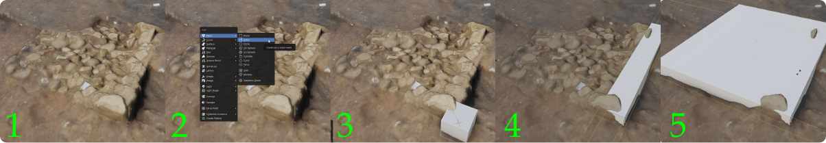
Sequence of steps for modelling a proxy in Blender. — Fig. 45 The proxy modelling process — five steps from base cube to fitted proxy.

Step 4: associate the proxy with its US

Once the proxy geometry is finished, select the corresponding US in the Stratigraphy Manager and use the associate control to bind proxy and US.

After binding, the proxy colour will reflect the colour scheme currently active in the EM Tools settings, and a closed-chain symbol will appear at the beginning of the corresponding row in the Stratigraphy Manager — a visual confirmation that proxy and US are successfully bound.

Colour schemes (EM vs. Periods, custom property-based mappings, saving and loading .emc files) are documented in Visual Manager.

Step 5: model the rest of the stratigraphy

Continue modelling every other US already prepared in the EM. The result is a single Blender scene in which every proxy is bound to a stratigraphic unit in the graph, classified by epoch, and ready to be combined with the higher-detail representation models in the next stage of the workflow.

For per-epoch selection, locking, visibility and soloing of the proxies you have just produced, see the Epochs Manager reference.